SPITZBERGEN
ROCKET (Instrumentation Notes)
1.
SENSOR
Electron spectrometer provides electron
detections parallel and perpendicular to Earth's magnetic field. The instrument
is swept in energy from 20keV down to eV in 32 energy levels. The instrument is
turned on just after 109.757seconds. Energy sweeps are about 0.246 seconds in
duration.
2.
SUSSEX CORRELATOR BOARD
Takes as inputs the two electron pulse
streams and processes each for HF correlations (Buncher 0-8MHz ), and LF
correlations (One-bit and multibit correlators at 0-3.33kHz and 0-10kHz).
Effectively ten 'virtual instruments':
2 directions x ( HF + 2 x ( LF frequency
ranges x 2 processing algorithms ) )
2.1
LF CORRELATOR
2.1.1
GENERAL
LF correlator data is available on an energy
sweep basis- no summation over sweeps.
Alternate energy sweeps are one-bit and multi-bit
correlators.
The top most energy is actually flyback and should
be ignored.
Alternate energy levels are 0-3.33kHz and 0-10kHz.
The data is transmitted as 10bit data with a bit
shift where data is above 1023 (10bits).
Sometimes (e.g. at 177.234s) the sweep
synchronisation slips and the default synchronisation value of 933 or a simple
2**n bit shift of this value is found in the data.
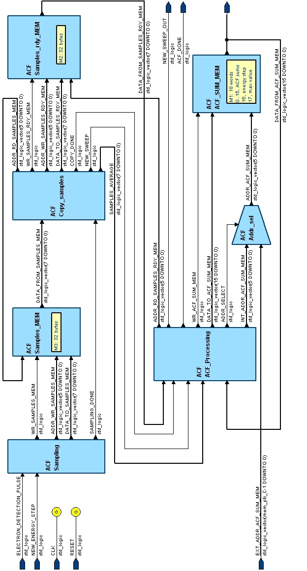
Data takes are 32 consecutive samples at 50us
(10kHz range) or 150us (3.33kHz range) with 16 point ACFs produced.
The energy step duration is sufficient for only one
data take and ACF at 0-3.33kHz on the odd energy levels. On the even, 0-10kHz,
energy levels three data takes with three ACF processes are made with the sum of
the three ACFs output at those levels.
2.1.2
ONE-BIT CORRELATOR
The one-bit correlator algorithms is the
standard algorithm as flown previously on AMPTE etc. 32 samples are converted to
32 bits depending on whether count sample is equal/above average or below, or
simple single counts where average below one. A simple 1-bit ACF is applied to
these 32 bits to give 16 lags.
The output values never invoke the bit shift
algorithm.
2.1.3
MULTI-BIT CORRELATOR
The 32 actual count samples are used directly
multiplying the samples to generate lags.
Each of the 16 lags is the sum of 16 products of
count sample pairs with the relevant lag. When the ACF includes values above
1023 the whole ACF is bit shifted down by an integral power of 2 to ensure all
values are <1023. The bit shift is transmitted and used in this program to
give the original value to a 9/10 bit accuracy. (There is no minimum
subtraction). When plotting in 2-D the minimum can be subtracted - solely for
the plotting- emphasizing any modulation. The zero lag of the multi-bit ACF can
be used to generate a crude electron spectrum versus time.
2.1.4
LF ACF FREQUENCY ANALYSIS
In this programme the ACFs are analysed by
comparison with a cosine wave with starting phase fixed at the lowest lag
according to the algorithm (Multi-bit includes zero lag, one-bit start at
lag=1). A truncation of the cosine is used to window the algorithm. Each ACF is
tested with 16 linearly separated frequencies from the maximum (10kHz or
3.33kHz) down to a minimum=maximum/16. At each test the ACF values (relative to
the ACF average- i.e. signed values) are multiplied by the corresponding value
of the (signed) truncated cosine wave. The sum of these products is compared
against the square root of the average ACF value and used for the spectral
plots. As a guide when looking at individual ACF the peak frequency band value
is also expressed as a percentage of the total spectral values.
2.2.
HF CORRELATOR
The buncher algorithm is performed on
adjacent pairs of energy levels to give 16 energy bands at 16 lags. The 8-bit
buncher values are accumulated over 0.523seconds - a (non integral) couple of
energy sweeps Unfortunately the
first few lags include the electronics dead time and register low values.
However at times in the flight the values exceed the 8 bit 255 telemetry limit
and by moving from low lags where there is no overflow it is possible to take
this overflow into account. Again the top most energy level includes flyback.
3.
DISPLAYS
The graphics displays have been made as user
friendly as possible with interactive plots. e.g. clicking on LF ACF 3-D
spectra/energy or 3-D lag/energy gives the relevant ACF as a 2-D plot, value
listing , and 2-D spectral plot.
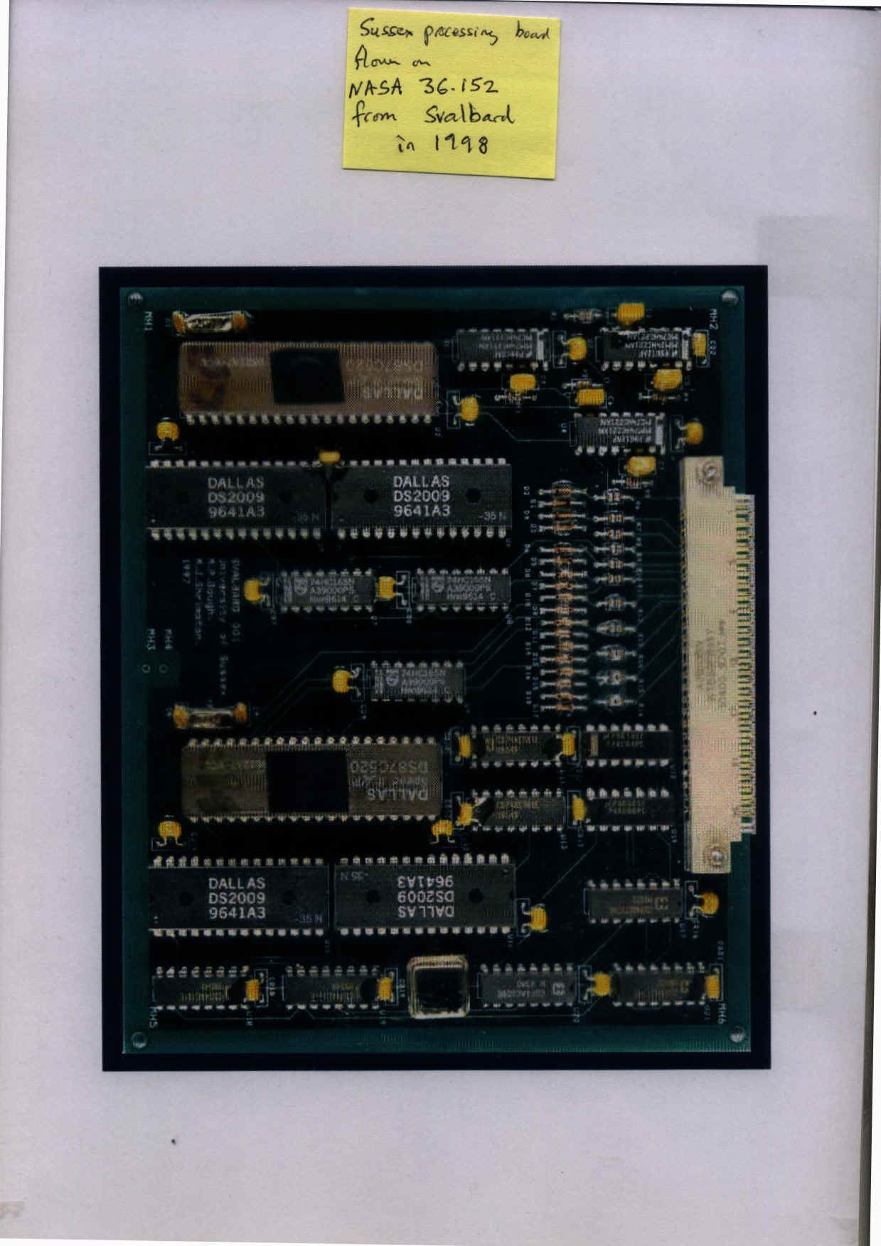
SVAL 8051
SVAL FPGA